Parallelization of learning of a neural network on Cpu-OpenMP and Gpu-NvidiaCUDA

06/08/2017 2295 words 11 minutes

Contents

Target

The goal is to optimize and parallelize a program provided in C for handwriting recognition by means of a back-propagation neural network. It is required that a parallelized version be produced on a processor that takes full advantage of the OpenMP compiler library and one that takes advantage of Nvidia Cuda technology. It is also required that particular attention be paid to memory access in the Cuda version.

Environment

The parallel version of the OpenMP program was achieved by developing and testing on a computer equipped with an Intel i7700k Kaby Lake and an ATI R9 290 video card (which is why the CUDA version was developed on another system).

The CUDA version was developed and tested on a Nvidia Quadro FX3800 1GB with Compute Capability of 1.3 coupled with a third generation Intel I3 Ivy Bridge. The IDE used is Atom, the makefile used is available together with the source code delivered. The analysis of the results was performed using the “perf” tool.

Monothread tuned version

Before parallelizing the program, it was useful to have an initial approach based on optimizing the existing code, remaining with a single execution flow. First, timers were placed between the various code macroblocks of the program to measure the computational weight of each one (data available in “nnml_analyzed-input.ml.log”).

It was immediately evident that the penultimate part, shown below, was the portion of the program that required the most time to execute (about 220 seconds).

Example of optimization on the penultimate macro block of code

 1
 2
 3
 4
 5
 6
 7
 8
 9
10
11
12
13
14
15
16
17
18
19
20
21
22
23
24
25
26
27
28
29
30
31
32
33
34
35
36
37
38
39
40
41
42
43
44


// before the tuning
for(h=NumHL; h>0; h--) { // cycle a
    for( j = 1 ; j <= nupl[h] ; j++ ) {  // cycle b
      DeltaWeightH2H[h-1][0][j] = alpha * DeltaWeightH2H[h-1][0][j];
      for( np = 0 ; np < NumPattern ; np++ ) { // cycle c
        p = ranpat[np];
        DeltaWeightH2H[h-1][0][j] += eta * DeltaH2H[h-1][p][j];
      }
    }
    for( j = 1 ; j <= nupl[h] ; j++ ) { // cycle d
      for( i = 1 ; i <= nupl[h-1] ; i++ ) {  // cycle e
        DeltaWeightH2H[h-1][i][j] = alpha * DeltaWeightH2H[h-1][i][j];
        for( np = 0 ; np < NumPattern ; np++ ) { // cycle f
          p = ranpat[np];
          DeltaWeightH2H[h-1][i][j] += eta * ((h>1)?H2H[h-2][p][i]:Input[p][i-1]) * DeltaH2H[h-1][p][j];
       }
      }
    }
  }
// after the tuning
for(h=1; h<=NumHL; h++) { // cycle a
    i_max = nupl[h-1];
    j_max = nupl[h];
    for( i = 0 ; i <= i_max ; i++ ) { // cycle b
      pointer32 = DeltaWeightH2H[h-1][i];
      for( j = 1 ; j <= j_max ; j++ )  //
        pointer32[j] *=alpha;
    }
    for( np = 0 ; np < NumPattern ; np++ ) { // cycle f
      p = ranpat[np];
      DeltaH2H_h1_p = DeltaH2H[h-1][p];
      factor_x = ((h>1)?H2H[h-2][p]:Input[p]);
      pointer32 = DeltaWeightH2H[h-1][0];
      for( j = 1 ; j <= j_max ; j++ ) 
        pointer32[j] += eta * DeltaH2H_h1_p[j];
      for( i = 1 ; i <= i_max ; i++ ) { // cycle e
        pointer32 = DeltaWeightH2H[h-1][i];
        factor_x_indexed = factor_x[((h>1)?i:i-1)] * eta;
        for( j = 1 ; j <= j_max ; j++ )  // cycle d
          pointer32[j] += factor_x_indexed * DeltaH2H_h1_p[j]; 
      }
    }
  }

The first optimization was to move the for “f” loop before “d”, in order to allow the processor to exploit the cache and avoid jumping from one point to another in a vast array (note that DeltaH2H and H2H have “p” as the second dimension, not the last one; because of this therefore by placing the innermost loop on the “p”, at each iteration the processor works on spatially distant portions of memory).

This change alone made it possible to reduce the execution time by almost 150 seconds and is just one example of how all sections of the code have been worked on, divided by numbered timers to identify any sectoral improvements following changes.

In fact, much of the optimization of the code has been based on optimizing access to the cache or reducing the number of operations required in the following ways:

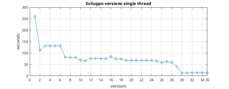
Going to change the order of inclusion of for loops based on the variables to be updated or read (versions 2, 7, 17, 22).
Using where necessary temporary support variables to be updated within cycles and then saved in memory, avoiding needlessly updating this memory value at each iteration (3, 5, 10, 11, 13, 23, 31, 32, 33 , 34).
Merging or splitting in two for loops to optimize memory access: cycle fusion or splitting (13, 14, 15).
Reducing the statements to be executed repeatedly inside the fors, for example by exploiting the associativity of the operations +,* (26,27,28,29).
Enabling optimization flags Ofast (includes O3), -funroll-loops, -fbounds-check, -funswitch-loops in the makefile (30).

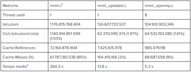
As can be seen from the version graph, the development of this optimized version has made it possible on our system to reduce execution times from more than 250 seconds to just over 10.

OpenMP version

The parallel OpenMP version was developed from the optimized version, as it was a good basis to parallelize given the number of improvements already made.

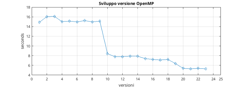
Versions 10, 11 constitute the parallelization of the central block of the program. In this phase it was necessary to use the primitive “omp atomic” to preserve the integrity of the global value of the error. The delay caused by the serialization of the error update operation is offset by a considerable advantage in execution times due to the parallelization of the for loops. Furthermore, where necessary, extensive use has been made of features such as the “omp simd” (which allows the vectorization of single thread cycles) and the “omp reduction” (for example to optimize cycles of adding a variable).

Much attention has also been paid to the “visibility” of variables in OpenMP parallel code blocks. The goal was to minimize the interaction between threads via variables (declaring variables as private or firstprivate), thus maximizing parallelism.

The initialization part of the program, during which files are read, has been parallelized using the “omp task” function, allowing a small gain on execution time (5, 12, 13, 14).

The penultimate optimized loop, discussed in the previous chapter, has been modified to avoid the use of atomic operations which would have negated the benefit of parallel execution. Thanks to the work carried out, however, an improvement in performance was also obtained in that portion of the code (20, 21, 22, 23).

Finally, different types of scheduler for the “omp parallel for” blocks were tested and the one that returned the best results on the test system was chosen (24).

Cuda version

The CUDA version was developed from “nnml_openmp.c” and “nnml_updated.c”. Using the subdivision into portions of code already used for development, we proceeded by adding a CUDA kernel with equivalent functionality to each block and with invocations of copy functions towards the device and from the device before and after gpu execution, in so as to be able to verify the correct implementation on the video card of the analyzed portion.

Due to this working method which has seen CPU code side by side with GPU code, and to the fact that the system on which it was developed is much less performing than the one used for the other parts (the function that verifies the correctness of the output of the program takes much longer, it would have slowed down development), it was not possible to keep a log of the development of the application.

The architectural decision to divide the program into numerous kernels was dictated both by the greatest possible performance by choosing the optimal number of threads for each portion of code, and by the maximum execution time of a kernel provided by the video card driver before raising a timeout exception.

Management of Arrays

As per “Best Practice” Cuda, the multidimensional arrays used have been implemented as one-dimensional arrays, going to “flatten” them. This choice has led to the need to calculate the correct positioning of multidimensional cells projected onto a single large 1d array. Furthermore, some 3-dimensional vectors used by the algorithm provided are not made up of lists of homodimensional matrices, but with matrices of different lengths, complicating any calculation of the index on the flattened structure (the cells have been written in a single large vector, placing the rows one after another forming matrices, also one after another forming the 3d vector).

The problem was solved with the introduction of data structures that could incorporate this complexity:

 1
 2
 3
 4
 5
 6
 7
 8
 9
10
11
12


struct Vector_3D {
    VECTOR_TYPE * vector;
    int x_dim;
    int y_dim[MAX_SIZE_VECTOR];
    int z_dim[MAX_SIZE_VECTOR];
  };
struct Vector_2D {
    VECTOR_TYPE * vector;
    int rows;
    int cols;
  };

The vector pointer points to the one-dimensional array (on gpu or cpu) of the flattened multidimensional array.

In the two-dimensional case the number of lines and columns were indicated, while in the 3D case “x_dim” was defined as the number of 2D matrices and two vectors “y_dim” and “z_dim” respectively array of number of lines and columns of the matrices contained in the 3D array.

The advantage of having incorporated all the information about a vector within the struct lies in the possibility of constructing methods that can return the requested index, passing only the struct in question and the requested coordinates as a parameter, not bothering to call for each invocation of the function the real dimensions of the vector. In the same way, functions for copying in both directions between device and host have been implemented which need only the structs of the arrays as parameters.

 1
 2
 3
 4
 5
 6
 7
 8
 9
10
11
12
13


__device__ static inline int index_3D_gpu
         (struct Vector_3D v, int x, int y, int z){
    int x_t = x;
    int index = y * v.z_dim[x] + z;
    for (;x_t>0;x_t--){
      index += v.z_dim[x_t-1] * v.y_dim[x_t-1];
    }
    return index;
  }
  __device__ static inline int index_2D_gpu
                       (struct Vector_2D matrix, int x, int y){
    return x*(matrix.cols)+y;
  }

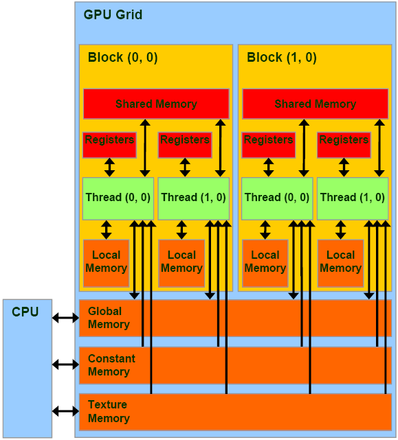
GPU Memories GPU

[http://docs.nvidia.com/cuda/cuda-c-programming-guide/index.html#device-memory-accesses](http://docs.nvidia.com/cuda/cuda-c-programming-guide/index.html#device-memory-accesses)

Shared Memory

To ensure excellent performance in kernels that require operations such as matrix multiplication, with a large number of accesses to global memory, extensive use of “Shared Memory” has been made. Following what was explained in the classroom and available in the Cuda documentation on Shared Memory, the “Tiled” algorithm was implemented in kernel 0, 1, 7, 8. The idea is to preload portions of matrices in Shared Memory, in a parallel way between thread of the same block, to then go and perform the requested operation by exploiting the speed of the Shared Memory (and the parallel access that this memory guarantees if without conflicts).

In Kernel 2, 3, given the limited size of some input vectors, it was possible to load the entire matrix directly into Shared Memory.

Constant Memory

The “Constant Memory” has proved useful in the case of read-only variables, such as integers passed in input, accessed simultaneously by different threads, even of different blocks. For a “half warp” reading a variable in Constant Memory is a parallel operation as fast as reading from a register, with the advantage of not having to request a register for each thread.

It has been used in almost all 11 kernels for constants like “NumPattern”, “NumHL”, ”NumOutput”.

Texture Memory

The Constant Memory is a memory that allows very fast reading operations, but is characterized by a small capacity (currently 64KB). Some vectors passed as input to the program such as “ranpat” and “nupl” are accessed by the program massively by threads and always in read mode.

Unfortunately, the excessive size of the first and their unknown length at compile time made it impossible to allocate them in Constant Memory.

Luckily the CUDA architecture provides the “Texture Memory” which allows dynamic allocation, it is common for all blocks (unlike the Shared Memory, so there is no data replication), it uses a cache on the chip (allowing reads very fast) and offering excellent performance when accessing spatially close data (these vectors are accessed by many threads simultaneously cycling over them).

Atomic Operations

As for the OpenMP version, the use of the atomic addition operation was made necessary for the calculation of the global error. Given the desire to keep the program compatible with deprecated versions of Compute Capability such as 1.3, an implementation suggested by the Cuda documentation of the “atomicAdd” was used, which exploits atomic functions available on this version of CC.

To lessen the negative impact that an atomic operation not natively supported by the hardware could have on execution time, atomic addition was built into a kernel that does the addition by reduction first within the various thread blocks, and only as a final reduction does it use the atomic primitive.

Checking the correctness of the program

In order to verify the integrity of the calculation modules of the original program throughout the development phase, the kernels were accompanied by the original cpu code, in order to compare inputs and outputs. As further proof of correctness, the script provided with the trace for verifying the generated output files was used.

Another useful tool for checking the Cuda program was “cuda-memcheck”, available in the Cuda toolkit, which can report any unauthorized memory access, a symptom of a malfunction or incorrect implementation.

Repository

https://gitlab.com/Ablablab/multi-many-core-1617

References

[1] http://www.openmp.org/
[2] http://www.nvidia.it/object/cuda-parallel-computing-it.html
[3] Compiled without compiler optimizations.
[4] Measured by linux time function (low accuracy), average of 10 runs.
[5] The c99 standard solves the problem by allowing structs to be declared with arrays of variable size int vec . For compatibility, it was decided to declare a maximum size statically.
[6] http://docs.nvidia.com/cuda/cuda-c-programming-guide/index.html#shared-memory
[7] http://docs.nvidia.com/cuda/cuda-c-programming-guide/index.html#device-memory-accesses
[8] http://docs.nvidia.com/cuda/cuda-c-programming-guide/index.html#atomic-functions